Spark Execution Plan Part 1
Introduction
Those coming from the Ab Initio world are accustomed to having complete control over the data pipeline from the very beginning. The graph clearly shows how data is read, which components are used with which parameters, when partitioning occurs, and when a new phase of execution begins. Every step in the processing workflow is configured manually and is fully traceable.
In Spark, this feels a bit different at first. You write code and execute transformations and actions, but the optimizer in the background decides how the code is actually executed. When data is actually read, which join strategy is chosen, and whether a shuffle occurs can only be controlled indirectly.
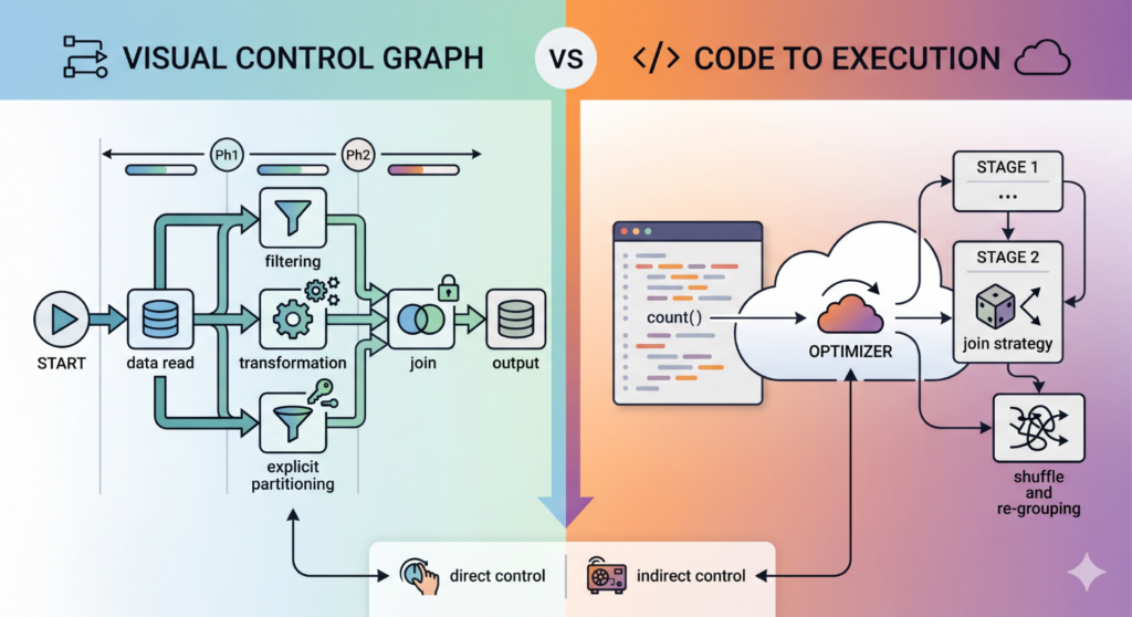
Visualization created with the help of AI (Gemini)
The background processes that run in Spark are, of course, no accident, but rather the result of a multi-stage optimization process. Spark first translates the code into a logical plan and then transforms it into a physical execution plan.
This physical implementation plan, the so called Execution Plan, is the actual execution reality of the pipeline. If you want to truly understand Spark and specifically influence its performance, this is exactly where you need to start: with the execution plan.
Following this theoretical classification, the crucial question arises:
What does this execution plan look like in practice?
Execution Plan in Practice
To make this clearer, let’s look at a concrete example. We’ll recreate a typical data engineering scenario: A large transaction table is joined with a customer table, and then some business calculations and aggregations are performed.
In Ab Initio, this use case would be modeled as a clearly structured graph: data sources, join components, transformation steps, and aggregation. In Spark, a handful of lines of code are all it takes to achieve this. However, it then becomes clear how Spark generates a multi-stage execution plan with multiple phases and data movements from what appears to be a simple ETL pipeline.
For our use case, we are creating a large transaction table with 30 million rows and a customer table with approximately 1 million customers. In addition, we are intentionally including a dominant join key: 70% of the transactions belong to a “VIP_CUSTOMER”.
					spark.conf.set("spark.sql.autoBroadcastJoinThreshold", -1)
spark.conf.set("spark.sql.adaptive.enabled", "false")

df_transactions = (
    spark.range(30_000_000)
    .withColumnRenamed("id", "transaction_id")
    .withColumn(
        "customer_id",
        F.when(F.rand() < 0.7, F.lit("VIP_CUSTOMER"))
         .otherwise((F.rand() * 1_000_000).cast("string"))
    )
    .withColumn("amount", F.rand() * 1000)
)

df_customers = (
    spark.range(1_000_000)
    .withColumnRenamed("id", "customer_id")
    .withColumn("customer_id", F.col("customer_id").cast("string"))
)

vip = spark.createDataFrame([Row(customer_id="VIP_CUSTOMER")])
df_customers = vip.union(df_customers)

total_sum = (
    df_transactions
    .join(df_customers, "customer_id")
    .withColumn("processed_amount", heavy_udf(F.col("amount")))
    .agg(F.sum("processed_amount"))
    .collect()
)
The Spark configuration was chosen deliberately:
- Broadcast joins are disabled. This means Spark cannot simply copy the much smaller customer table to all worker nodes during the join.
- Adaptive Query Execution is disabled. This allows us to see the basic physical plan without dynamic runtime adjustments.
The pipeline has been deliberately kept simple: two data sources, one join, and a final aggregation. However, as soon as an action such as .collect() is executed, Spark translates these few transformations into a complex physical execution plan. So it’s not enough to simply look at the code. Only the execution plan reveals exactly how the data is partitioned, which processes run in parallel, and how the join strategies are implemented.
The execution plan can be displayed using the following command:
total_sum.explain("formatted")
Due to its complexity, we are not showing the entire plan here, but only the parts of the execution plan that are most important for understanding it. The execution plan is best read from bottom to top.
					== Physical Plan ==

HashAggregate
+- Exchange
   +- HashAggregate
      +- Project
         +- BatchEvalPython
            +- SortMergeJoin
               :- Exchange hashpartitioning(customer_id, 8)
               +- Exchange hashpartitioning(customer_id, 8)
The key operators here are:
- Exchange hashpartitioning(customer_id, 8): This operator describes the partitioning of data based on the join key customer_id. Since broadcast joins are disabled, both sides of the join must be split using a shuffle based on the same partitioning key. In Ab Initio, this step corresponds to using a Partition By Key component, which also splits a data stream into multiple partitions based on a key field.
- SortMergeJoin: After partitioning the two sides, Spark performs the join using a SortMergeJoin. This efficient algorithm is rarely the problem; the real cost lies in the shuffle operation required to support it.
- BatchEvalPython: After the join, the Python UDF is executed. Spark cannot fully optimize this logic in the same way it does with native SQL expressions. The data must therefore be processed directly in Python, which introduces additional overhead. In Ab Initio, this would be comparable to a component such as Run Program, in which external code runs outside the highly optimized standard components.
- HashAggregate/Exchange: Aggregation now takes place in two steps. First, Spark aggregates locally per partition, then performs an additional exchange step in which the partial results are transferred to a worker node. The final aggregation step then takes place there.
The key difference between Ab Initio and Spark lies in their approach to building the transformation logic:
In Ab Initio, every aspect of the data flow is explicitly modeled: partitioning and join parameterization are part of the graph and are entirely controlled by the developer. In Spark, on the other hand, the developer merely describes the transformations, while the physical execution is generated by the optimizer at runtime and becomes visible in the execution plan.
That is precisely why the execution plan is the key tool for truly understanding Spark. It not only shows what happens, but more importantly, how it happens and where the actual costs arise. Those who can read it can identify shuffles, join strategies, and bottlenecks before they become a problem.
Outlook
Our use case also involves another critical factor: 70% of the data is concentrated on a single join key. This uneven distribution isn’t immediately apparent in the execution plan, but it can cause massive performance issues at runtime. In the next section, we’ll examine this very phenomenon, Data Skew , and how to address it.